library(ggcorrheatmap)
library(dplyr)
library(tidyr)    # For converting between long and wide formats
library(tibble)
library(patchwork)
Data is often in long format when working with ggplot2
and other functions in the tidyverse. The
gghm_tidy() and ggcorrhm_tidy() functions
provide a way to use the heatmap plotting functionality of
ggcorrheatmap with long format data. These functions (and
this article) assume that the user is familiar with the arguments of the
non-tidy versions of the functions.
Heatmaps
# Make some long format data using functions from
# the dplyr, tidyr, tibble packages
mtcars_long <- mtcars %>%
  as.data.frame() %>%
  # Move rownames into a column for long format conversion
  rownames_to_column("cars") %>%
  pivot_longer(cols = -cars, names_to = "vars", values_to = "vals")

head(mtcars_long)
#> # A tibble: 6 × 3
#>   cars      vars    vals
#>   <chr>     <chr>  <dbl>
#> 1 Mazda RX4 mpg    21
#> 2 Mazda RX4 cyl     6
#> 3 Mazda RX4 disp  160
#> 4 Mazda RX4 hp    110
#> 5 Mazda RX4 drat    3.9
#> 6 Mazda RX4 wt      2.62
When using gghm_tidy(), the names of the columns
containing the rows, columns, and values must be provided. These can be
unquoted, quoted, from variables, or indices.
value_column <- "vals"

# Provide column names unquoted, as index, and from variable
gghm_tidy(mtcars_long, rows = cars, cols = 2, values = !!value_column,
          # gghm arguments can be used (via ...)
          col_scale = "A", scale_data = "col")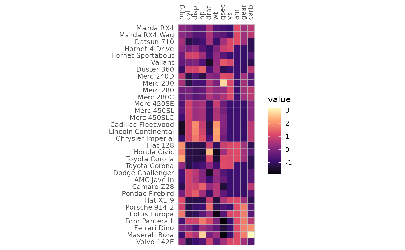
Columns containing annotations and cell labels can be specified in the same way.
# Make sure the annotations are unique
# (i.e. one row or column does not have two different annotation values)
set.seed(123)
row_key <- data.frame(cars = rownames(mtcars),
                      a = 1:nrow(mtcars),
                      b = sample(letters[1:3], nrow(mtcars), TRUE))
col_key <- data.frame(vars = colnames(mtcars),
                      c = 1:ncol(mtcars),
                      d = sample(LETTERS[1:2], ncol(mtcars), TRUE))

mtcars_long %>%
  # Add the row and column annotations
  left_join(row_key, by = "cars") %>%
  left_join(col_key, by = "vars") %>%
  # Add labels
  mutate(labs = 1:nrow(.)) %>%
  gghm_tidy(cars, vars, vals, labels = labs,
            annot_rows = c(a, b), annot_col = c(c, d),
            # gghm arguments
            legend_order = 1, cell_label_col = "white",
            cell_label_digits = 0, col_scale = "A",
            scale_data = "col", cell_label_size = 2,
            cluster_rows = TRUE, cluster_cols = TRUE)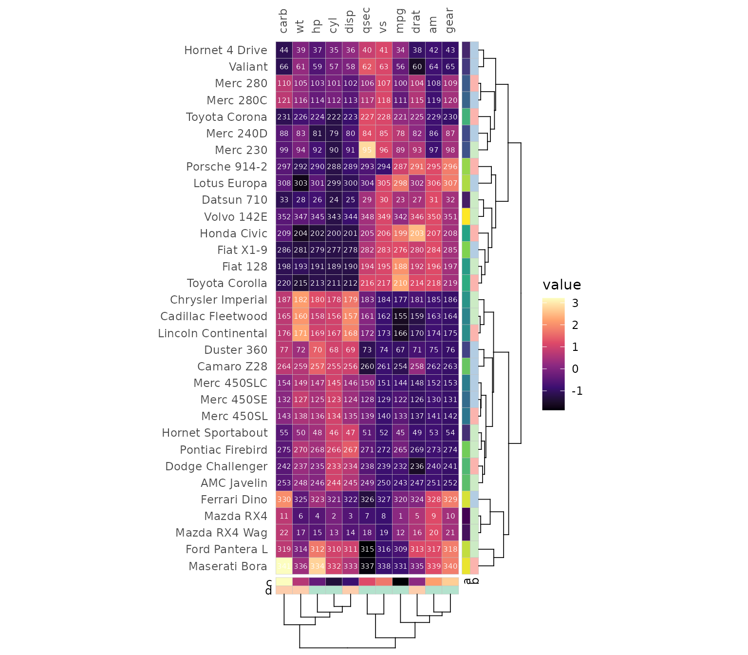
When introducing gaps the facet_rows and
facet_cols arguments allow for facet membership
specification using columns in the input. It is still possible to
specify the splits with the split_rows and
split_cols arguments for the same behaviour as in
gghm().
plt1 <- mtcars_long %>%
  # Use the annotations as facets
  left_join(row_key, by = "cars") %>%
  left_join(col_key, by = "vars") %>%
  # Change facet order for rows
  mutate(b = factor(b, levels = letters[1:3])) %>%
  gghm_tidy(cars, vars, vals,
            facet_rows = b, facet_cols = d)

plt2 <- gghm_tidy(mtcars_long,
                  cars, vars, vals,
                  split_rows = 16,
                  split_cols = 6)

plt1 + plt2
Correlation heatmaps
ggcorrhm_tidy() is the tidy version of
ggcorrhm(), although not all of the functionality is
available. By default, the input is assumed to contain correlation
coefficients (cor_in is TRUE). If
cor_in is FALSE the behaviour changes and some
arguments work differently.
The cor_long() function can be used to calculate
correlations from long format data. By default the output is in wide
format and can be passed to ggcorrhm().
ggcorrhm(
  cor_long(mtcars_long, cars, vars, vals, out_format = "wide"),
  # Specify that the input contains correlation values
  cor_in = TRUE
)
If desired, the correlation data can be returned in long format,
which can be given to ggcorrhm_tidy() to make a
heatmap.
mtcars_cor <- cor_long(mtcars_long, cars, vars, vals,
                       out_format = "long")

# Can also be done using tidyverse functions, something like
# mtcars_long %>%
#   pivot_wider(id_cols = "cars", names_from = "vars", values_from = "vals") %>%
#   column_to_rownames("cars") %>%
#   cor() %>%
#   # This part only needed if output should be long format
#   as.data.frame() %>%
#   rownames_to_column("row") %>%
#   pivot_longer(cols = -row, names_to = "col")

head(mtcars_cor)
#>    row col      value
#> 1  mpg mpg  1.0000000
#> 2  cyl mpg -0.8521620
#> 3 disp mpg -0.8475514
#> 4   hp mpg -0.7761684
#> 5 drat mpg  0.6811719
#> 6   wt mpg -0.8676594
ggcorrhm_tidy(mtcars_cor, row, col, value)
It is also possible to correlate two different matrices.
# Make another long format data
iris_long <- iris %>%
  # The dimensions of the two matrices must be compatible
  slice(1:32) %>%
  # Make unique names for the rows
  mutate(Species = make.names(Species, unique = TRUE)) %>%
  rename(species = Species) %>%
  # Convert to long format
  pivot_longer(cols = -species)

head(iris_long)
#> # A tibble: 6 × 3
#>   species  name         value
#>   <chr>    <chr>        <dbl>
#> 1 setosa   Sepal.Length   5.1
#> 2 setosa   Sepal.Width    3.5
#> 3 setosa   Petal.Length   1.4
#> 4 setosa   Petal.Width    0.2
#> 5 setosa.1 Sepal.Length   4.9
#> 6 setosa.1 Sepal.Width    3
# Correlate the two long format matrices
mi_cor <- cor_long(iris_long, species, name, value,
                   # The first one ends up in the rows and
                   # the second in the columns
                   mtcars_long, cars, vars, vals,
                   out_format = "long")

head(mi_cor)
#>            row col        value
#> 1 Sepal.Length mpg  0.000136181
#> 2  Sepal.Width mpg -0.162115780
#> 3 Petal.Length mpg  0.242985583
#> 4  Petal.Width mpg -0.052943516
#> 5 Sepal.Length cyl -0.107232949
#> 6  Sepal.Width cyl  0.166560421
ggcorrhm_tidy(mi_cor, row, col, value)
If the cor_in argument is FALSE,
ggcorrhm_tidy() will calculate the correlations instead.
Both options come with limitations.
cor_in is FALSE:
Cannot correlate two different matrices.
annot_rowsandannot_colsrequire different thinking as both will use the names from the column specified ascols.The
labelsargument works like ingghm(), taking a combination of TRUE and FALSE or a (wide format) matrix or data frame (and, additionally, NULL).
cor_in is TRUE:
Requires the correlation values to be pre-computed.
As all correlation calculations are skipped, p-values will not be computed and will also need to be calculated in advance. The
cor_long()function can help with this.The
labelsargument works like ingghm_tidy(), taking a column in the data.
# Give the non-correlation data
ggcorrhm_tidy(mtcars_long, cars, vars, vals,
              cor_in = FALSE, labels = TRUE)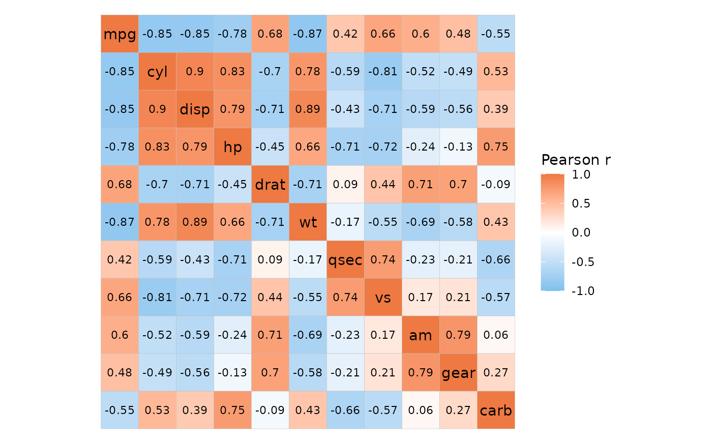
Like with gghm_tidy(), ggcorrhm_tidy() can
take arguments from ggcorrhm() for extra customisation.
# Annotation
cor_annot <- data.frame(.names = colnames(mtcars),
                        annot1 = 1:11, annot2 = 11:1,
                        annot3 = sample(letters[1:2], 11, TRUE),
                        annot4 = sample(LETTERS[1:3], 11, TRUE))

mtcars_cor_extra <- mtcars_cor %>%
  # Add row annotations
  left_join(select(cor_annot, .names, annot1, annot3),
            by = c("row" = ".names")) %>%
  # Add column annotations
  left_join(select(cor_annot, .names, annot2, annot4),
            by = c("col" = ".names")) %>%
  # Add labels
  mutate(labs = 1:nrow(.))
head(mtcars_cor_extra)
#>    row col      value annot1 annot3 annot2 annot4 labs
#> 1  mpg mpg  1.0000000      1      a     11      A    1
#> 2  cyl mpg -0.8521620      2      a     11      A    2
#> 3 disp mpg -0.8475514      3      b     11      A    3
#> 4   hp mpg -0.7761684      4      a     11      A    4
#> 5 drat mpg  0.6811719      5      a     11      A    5
#> 6   wt mpg -0.8676594      6      a     11      A    6
ggcorrhm_tidy(mtcars_cor_extra, row, col, value,
              annot_rows = c(annot1, annot3),
              annot_cols = c(annot2, annot4),
              labels = labs,
              cluster_rows = TRUE, cluster_cols = TRUE,
              layout = c("tl", "br"), mode = c("hm", "hm"),
              col_scale = c("A", "G"), cell_label_col = "white",
              legend_order = c(1, 2))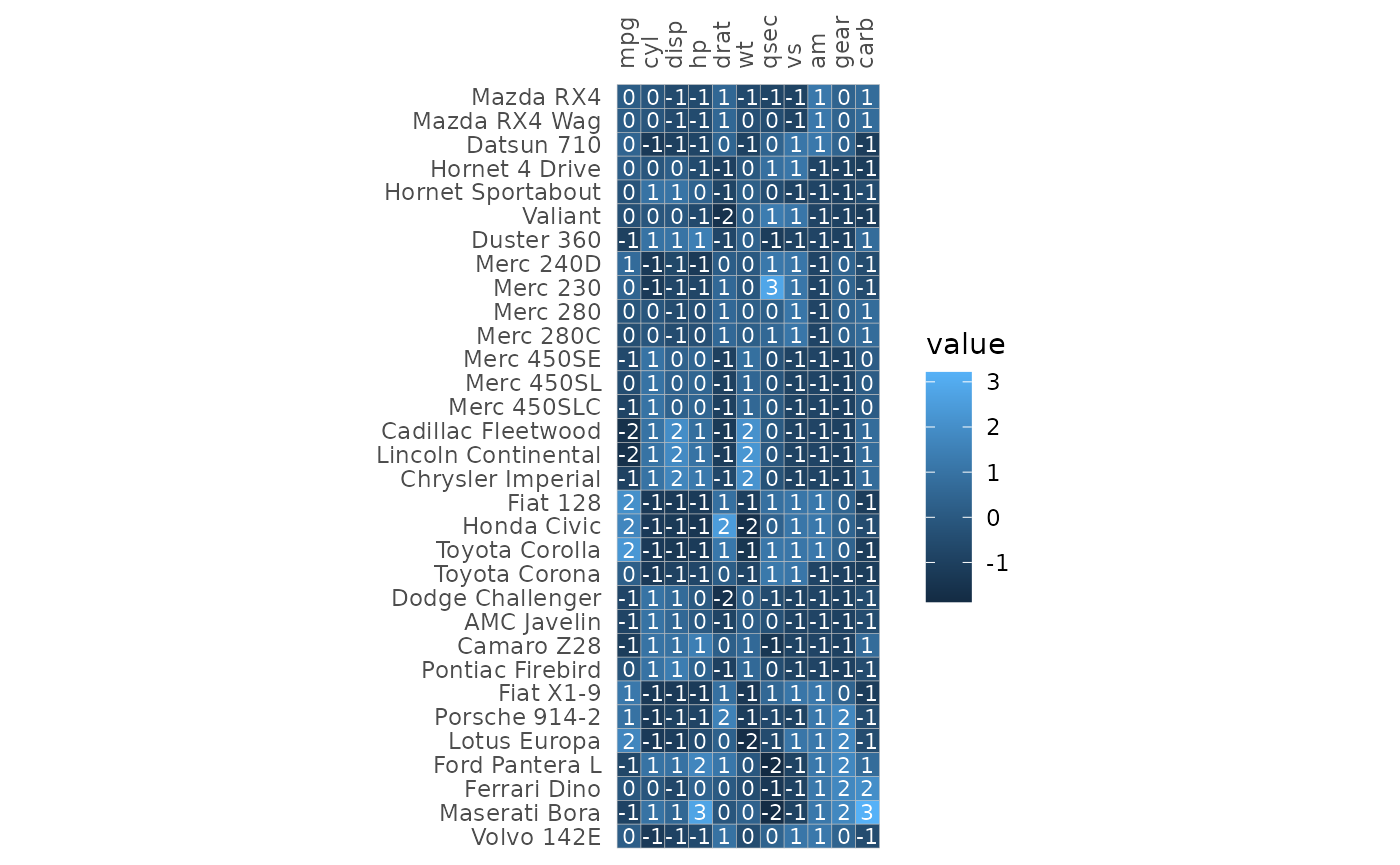
Cell labels and mixed layouts
When adding cell labels in gghm_tidy(), if the value
column and cell label column are the same the cell labels will be
affected by the scale_data argument.
gghm_tidy(mtcars_long, cars, vars, vals,
          labels = vals, scale_data = "col",
          cell_label_digits = 0, cell_label_col = "white")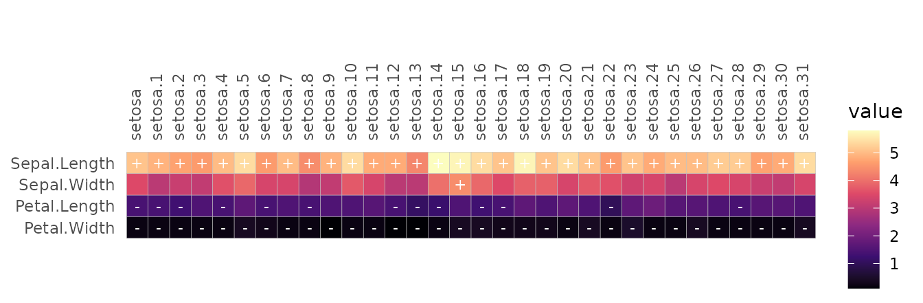
It is also convenient to make conditional cell labels when the data is in long format, such as using different labels depending on the cell values.
iris_long %>%
  mutate(labs = case_when(value < 1.5 ~ "-",
                          value > 4 ~ "+",
                          TRUE ~ "")) %>%
  gghm_tidy(name, species, value, labels = labs,
            col_scale = "A", cell_label_col = "white")
When working with mixed layouts, gghm() can take care of
labelling only one half of the heatmap. Since the tidy version just uses
the values in the specified labels column, a bit more work
is required.
For convenience, the add_mixed_layout() helper function
can add a column showing which values will end up in which triangle of a
mixed layout to help with labelling cells.
# Get long format data
df_long <- sapply(seq(-1, 0, length.out = 15), function(x) {
  seq(x, x + 1, length.out = 15)
}) %>% as.data.frame() %>%
  `colnames<-`(1:15) %>%
  rownames_to_column("a") %>%
  pivot_longer(cols = -a, names_to = "b") %>%
  # Add column saying which triangle each value is in
  add_mixed_layout(rows = a, cols = b, values = value,
                   layout = c("tl", "br"))

head(df_long)
#> # A tibble: 6 × 4
#>   a     b      value layout
#>   <chr> <chr>  <dbl> <chr>
#> 1 1     1     -1     tl
#> 2 1     2     -0.929 br
#> 3 1     3     -0.857 br
#> 4 1     4     -0.786 br
#> 5 1     5     -0.714 br
#> 6 1     6     -0.643 br
df_long %>%
  # Add labels only for the top left part
  mutate(label = if_else(layout == "tl", "+", "")) %>%
  gghm_tidy(a, b, value, labels = label,
            # Make sure to use the same layout as in add_mixed_layout
            # to avoid confusion
            layout = c("tl", "br"), mode = c("hm", "hm"),
            col_scale = c("G", "A"), cell_label_col = "white")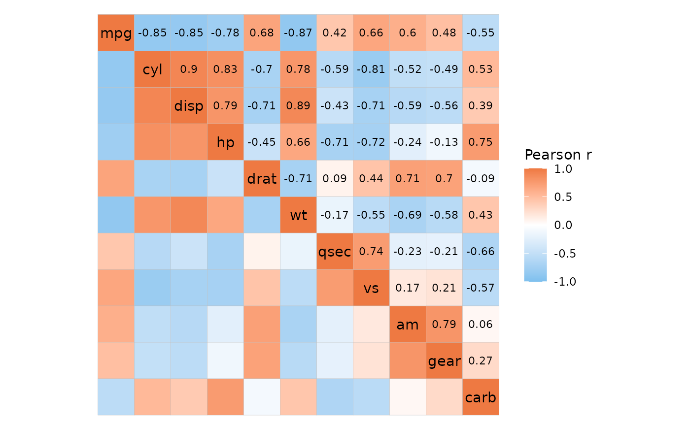
ggcorrhm_tidy() works similarly if cor_in
is TRUE. If FALSE, the labels
argument works like in ggcorrhm(), taking a wide format
matrix/data frame or a combination of TRUE and
FALSE.
# `cor_in` is `TRUE`
mtcars_cor %>%
  # Add layout column
  add_mixed_layout(layout = c("bl", "tr")) %>%
  # Add cell labels
  mutate(lab = if_else(layout == "tr", value, NA)) %>%
  ggcorrhm_tidy(row, col, value, labels = lab,
                cor_in = TRUE,
                layout = c("bl", "tr"), mode = c("hm", "hm"))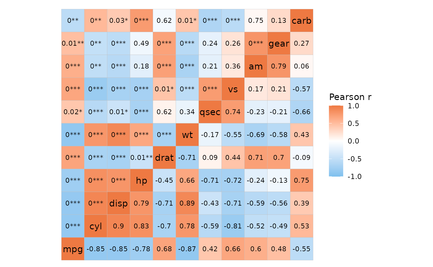
P-values
In ggcorrhm_tidy(), if cor_in is
FALSE, the p_values argument works like in
ggcorrhm() and can deal with mixed layouts.
ggcorrhm_tidy(mtcars_long, cars, vars, vals, cor_in = FALSE,
              layout = c("tl", "br"), mode = c("hm", "hm"),
              labels = TRUE, p_values = c(TRUE, FALSE),
              # P-values top left, correlation values bottom right
              cell_label_p = c(TRUE, FALSE))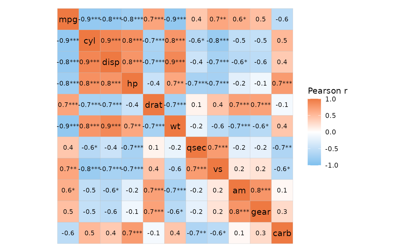
If cor_in is TRUE, the labels are drawn
directly from a column in the data, which means that the labels have to
be made in advance. To help with this, the cor_long
function has some extra p-value functionality.
mtcars_long %>%
  cor_long(cars, vars, vals,
           out_format = "long",
           p_values = TRUE,
           # Multiple testing adjustment
           p_adjust = "bonferroni",
           # Thresholds for symbols based on adjusted p-values
           p_thresholds = c("***" = 0.001, "**" = 0.01, "*" = 0.05, 1),
           # 'p_sym_add' takes a column and adds to the symbols for quick combining
           # One of 'values', 'p_val', and 'p_adj'
           p_sym_add = "value",
           # 'p_sym_digits' changes the number of decimals
           # displayed in the p_sym
           p_sym_digits = 1) %>%
  # The output contains the columns 'row', 'col', 'value',
  # 'p_val', 'p_adj', and 'p_sym'
  ggcorrhm_tidy(row, col, value, labels = p_sym)
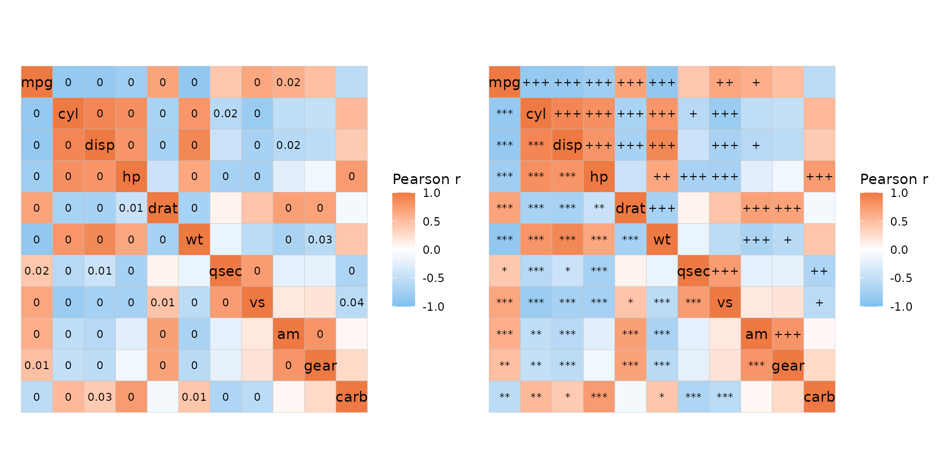
Combine this with add_mixed_layout for more control in
mixed layouts. Below is an example of showing unadjusted and adjusted
p-values in different triangles of the heatmap.
plt_dat <- mtcars_long %>%
  # Add p-values
  cor_long(cars, vars, vals, out_format = "long",
           p_values = TRUE, p_adjust = "bonferroni") %>%
  # Add layout
  add_mixed_layout(layout = c("tr", "bl"))

plt1 <- plt_dat %>%
  # Make custom labels with adjusted p-values in the
  # top right and unadjusted in the bottom left
  # but only display if < 0.05
  mutate(labs = case_when(layout == "tr" & p_adj < 0.05 ~ round(p_adj, 2),
                          layout == "bl" & p_val < 0.05 ~ round(p_val, 2),
                          TRUE ~ NA)) %>%
  ggcorrhm_tidy(row, col, value, labels = labs,
                cor_in = TRUE)

plt2 <- plt_dat %>%
  # Make symbol labels instead
  mutate(p_star = as.character(symnum(p_val, c(0, 0.001, 0.01, 0.05, 1),
                                      c("***", "**", "*", ""))),
         p_adj_star = as.character(symnum(p_adj, c(0, 0.001, 0.01, 0.05, 1),
                                          c("+++", "++", "+", ""))),
         labs = case_when(layout == "tr" & p_adj < 0.05 ~ p_adj_star,
                          layout == "bl" & p_val < 0.05 ~ p_star,
                          TRUE ~ "")) %>%
  ggcorrhm_tidy(row, col, value, labels = labs,
                cor_in = TRUE)

plt1 + plt2