Clustering

library(ggcorrheatmap)
library(dplyr)
library(dendextend)
library(patchwork)

Heatmap rows and columns are clustered if the cluster_rows and cluster_cols arguments are set to TRUE. Distance measure and clustering method can be specified with the cluster_distance and cluster_method arguments, passed on to the stats::dist() and stats::hclust() functions, respectively.

ggcorrhm(mtcars, cluster_rows = TRUE, cluster_cols = TRUE)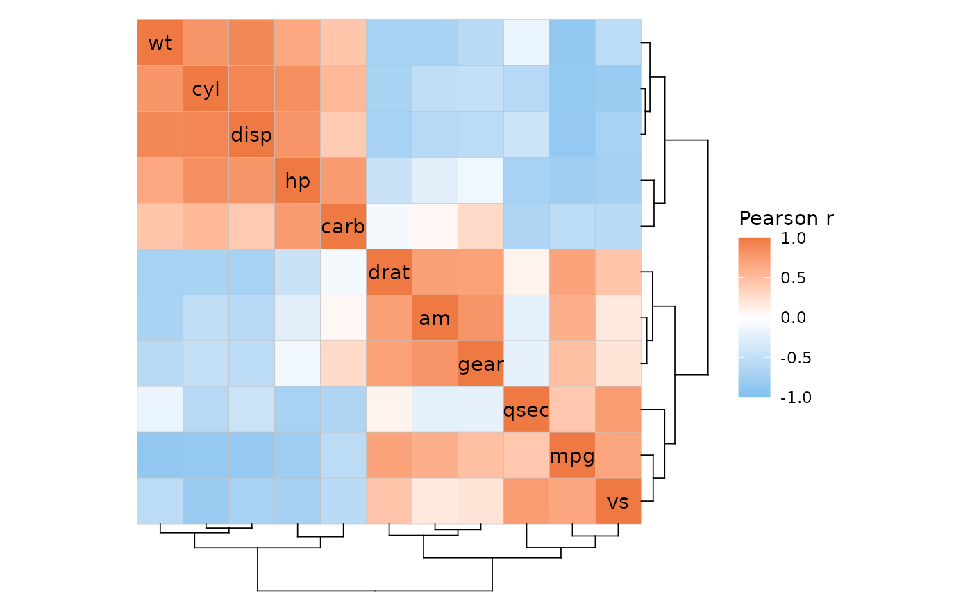

A correlation heatmap of the columns in the mtcars data. The cells are filled with colours ranging from blue (-1) to white (0) to red (1). The rows and columns have been clustered and dendrograms are drawn to the right and below the heatmap.

The cluster_rows and cluster_cols arguments can also be hclust or dendrogram objects if more control is required.

Dendrogram position

The positions of the dendrograms can be changed with the dend_rows_side (‘left’ or ‘right’) and dend_cols_side (‘top’ or ‘bottom’) arguments. For triangular layouts the dendrograms are placed on the non-empty sides of the heatmap.

# The dendrogram sides can be adjusted with the 'dend_rows_side' and 'dend_cols_side' arguments
plt1 <- ggcorrhm(mtcars, cluster_rows = TRUE, cluster_cols = TRUE,
                 dend_rows_side = "left", dend_cols_side = "top")

# Dendrograms can be hidden by setting 'show_dend_rows' and/or 'show_dend_cols' to FALSE
plt2 <- ggcorrhm(mtcars, cluster_rows = TRUE, cluster_cols = TRUE, layout = "bl",
                 show_dend_rows = FALSE, dend_cols_side = "top")

plt1 + plt2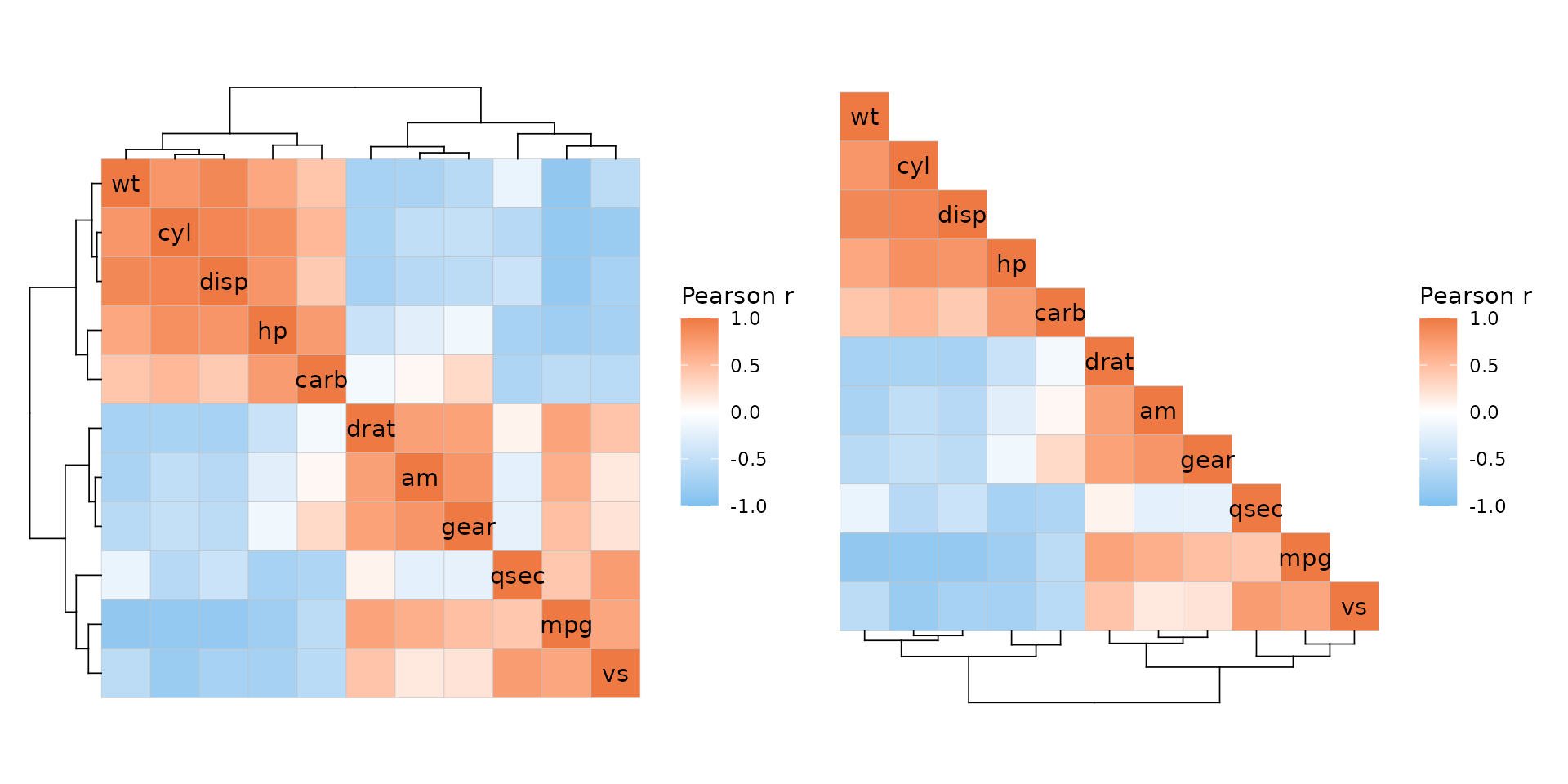

Two mtcars correlation heatmaps. The first one has the dendrograms on the top and left. The second plot has only drawn the bottom left triangle of the matrix and there is a dendrogram on the bottom.

If annotation and a dendrogram are on the same side, the dendrogram is moved to make place for the annotation.

annot <- data.frame(.names = colnames(mtcars), a = 1:11)
ggcorrhm(mtcars, cluster_rows = TRUE, cluster_cols = TRUE,
         annot_rows_df = annot, annot_cols_df = annot,
         dend_rows_side = "left")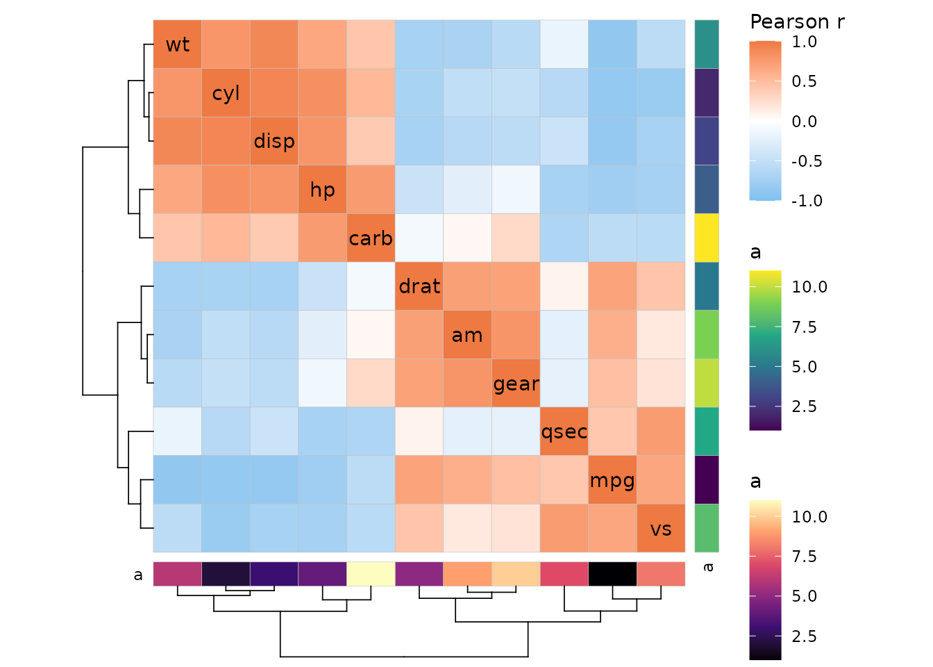

Changing how the dendrograms look

The dend_col, dend_dist, dend_height, dend_lwd, and dend_lty arguments change the colour, distance to the heatmap, height (scaling), linewidth, and linetype of the dendrograms, respectively.

ggcorrhm(mtcars, cluster_rows = TRUE, cluster_cols = TRUE,
         dend_col = "cyan", dend_height = 2, dend_lwd = 1, dend_lty = 2)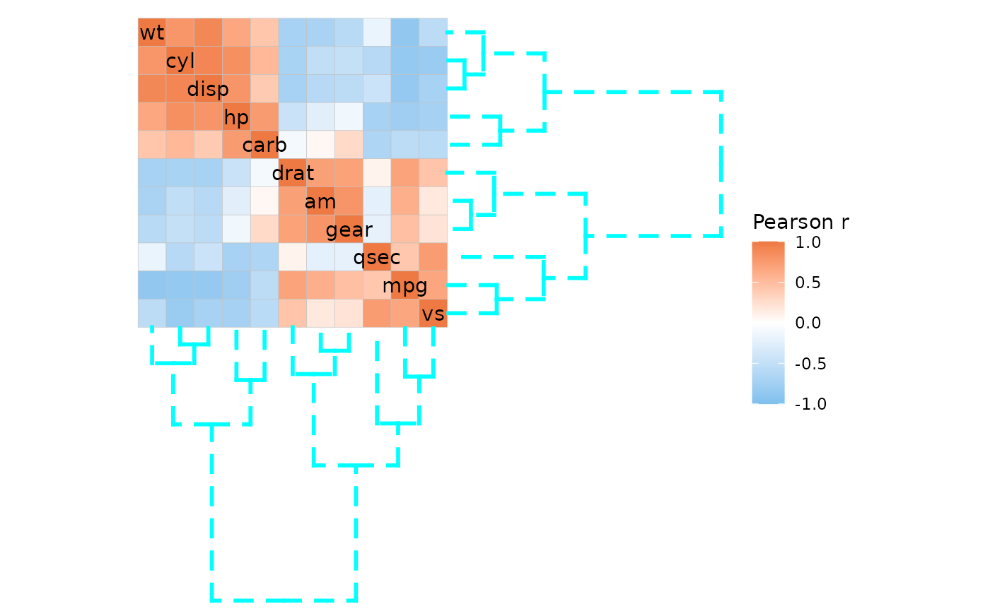

Correlation heatmap of mtcars with clustered rows and columns. The row and column dendrograms are longer and thicker than before, coloured cyan and dashed.

To apply these changes to only one of the dendrograms, use the dend_rows_params and dend_cols_params arguments. These arguments take a named list containing one or more of col, dist, height, lwd, and lty.

ggcorrhm(mtcars, cluster_rows = TRUE, cluster_cols = TRUE,
         dend_rows_params = list(col = "cyan", height = 2),
         dend_cols_params = list(lwd = 1, lty = 2, dist = 1))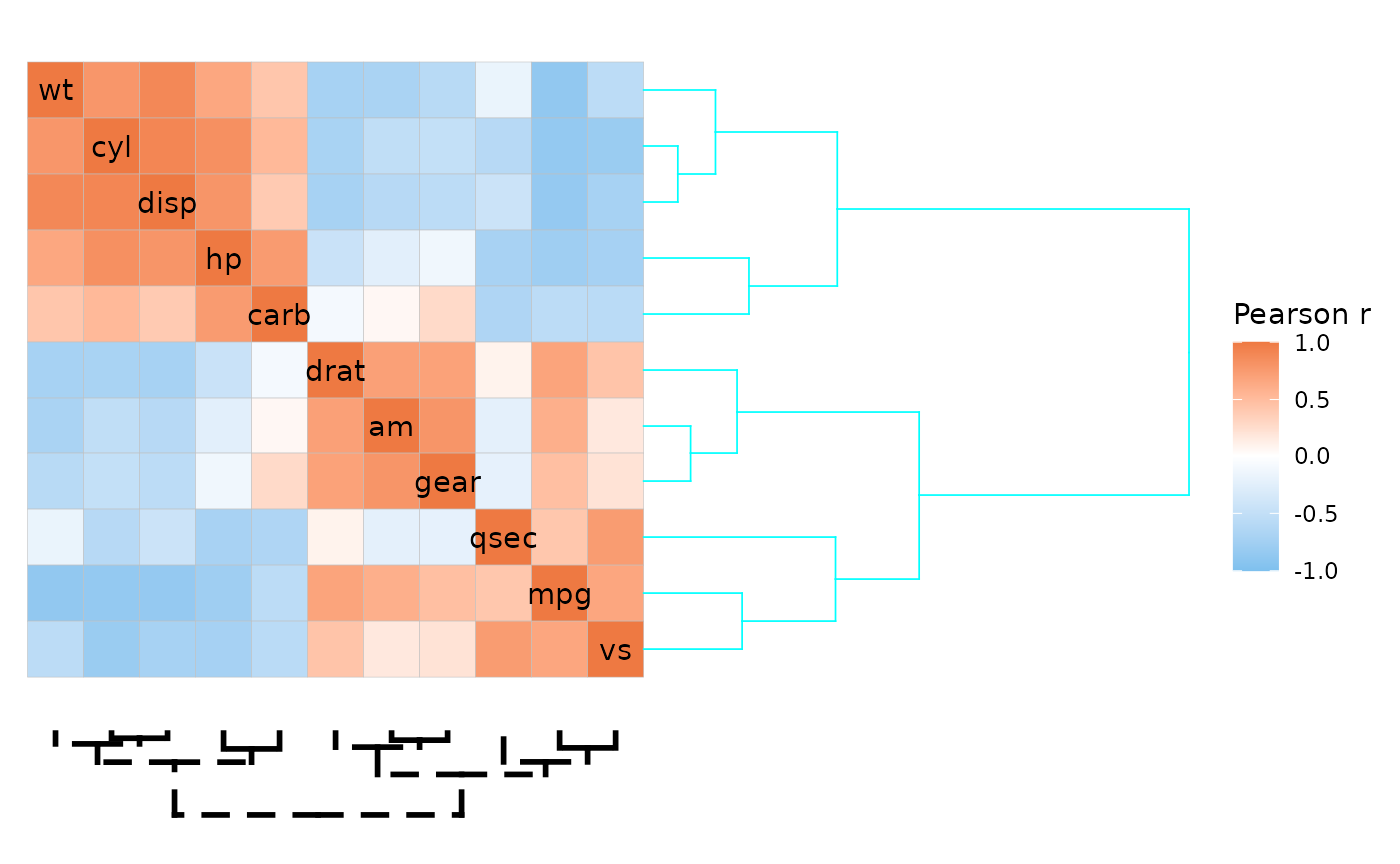

mtcors correlation heatmap with clustered rows and columns. The row dendrogram is tall and cyan like the previous plot, but solid and not thicker than normal. The column dendrogram is the default height and colour (black) but thick and dashed. There is a gap the size of one heatmap cell between the column dendrogram and the heatmap.

More customisation using `dendextend`

Finer customisation of dendrograms can be done with the dend_rows_extend and dend_cols_extend arguments. These use the dendextend package to change the dendrogram appearance. The input can be either a named list of lists, where each element is named after the dendextend function to use and contains a list of the arguments to pass, or a functional sequence (fseq object) that strings together the functions to use. A few examples are shown below, see the dendextend vignette vignette("dendextend", package = "dendextend") for more details on how to use its functions.

# List method
ggcorrhm(mtcars, cluster_rows = TRUE, cluster_cols = TRUE, dend_height = 1,
         # Multiple elements can use the same function as lists don't require unique names
         dend_rows_extend = list(
           set = list("branches_k_col", k = 3),
           set = list("branches_lty", c(1, 2, 3))
         ),
         # NULL or empty list if no arguments are to be passed
         dend_cols_extend = list(
           highlight_branches_lwd = list(values = seq(1, 4)),
           highlight_branches_col = list()
         ))
#> Loading required namespace: colorspace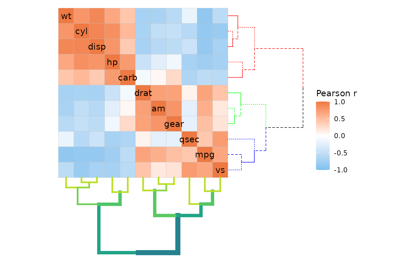

A clustered mtcars correlation heatmap again. The row dendrogram alternates between black, red, and green, as well as solid, dashed, and dotted. The column dendrogram starts thick and gets gradually thinner as it moves toward the heatmap. The colour comes from the viridis scale and shifts along the height of the dendrogram.

# The equivalent call using the fseq method
# library(dplyr)
# library(dendextend)
# ggcorrhm(mtcars, cluster_rows = TRUE, cluster_cols = TRUE,
#          dend_rows_extend = . %>%
#            set("branches_k_col", k = 3) %>%
#            set("branches_lty", c(1, 2, 3)),
#          dend_cols_extend = . %>%
#            highlight_branches_lwd(values = seq(1, 4)) %>%
#            highlight_branches_col())

It is also possible to display the nodes of the dendrograms.

# Get clustered labels
clust <- hclust(dist(cor(mtcars)))
clust_lab <- clust$labels[clust$order]

ggcorrhm(mtcars, cluster_rows = TRUE, cluster_cols = TRUE, dend_height = 1,
         # Here using the fseq method
         dend_rows_extend = . %>%
           # More on customising segments
           # Can specify branches to affect by labels using the 'by_labels_branches_*' options
           set("by_labels_branches_col", value = clust_lab[1:5], TF_values = "red") %>%
           set("by_labels_branches_lty", value = c("drat", "vs"), TF_values = 3) %>%
           set("by_labels_branches_lwd", value = clust_lab[6:11], TF_values = 1) %>%
           # Node and leaf options
           # Specify all nodes before leaves so the leaf options are not overwritten
           # pch must be specified for a node to be drawn
           set("nodes_pch", 19) %>%
           set("nodes_cex", 2) %>%
           set("nodes_col", "orange") %>%
           set("leaves_pch", 21) %>%
           set("leaves_cex", 3) %>%
           set("leaves_col", "purple"),
         dend_cols_extend = . %>%
           highlight_branches_col() %>%
           # Node options
           set("nodes_pch", c(15, 16, 17)) %>%
           set("nodes_cex", 2:4) %>%
           set("nodes_col", 1:5))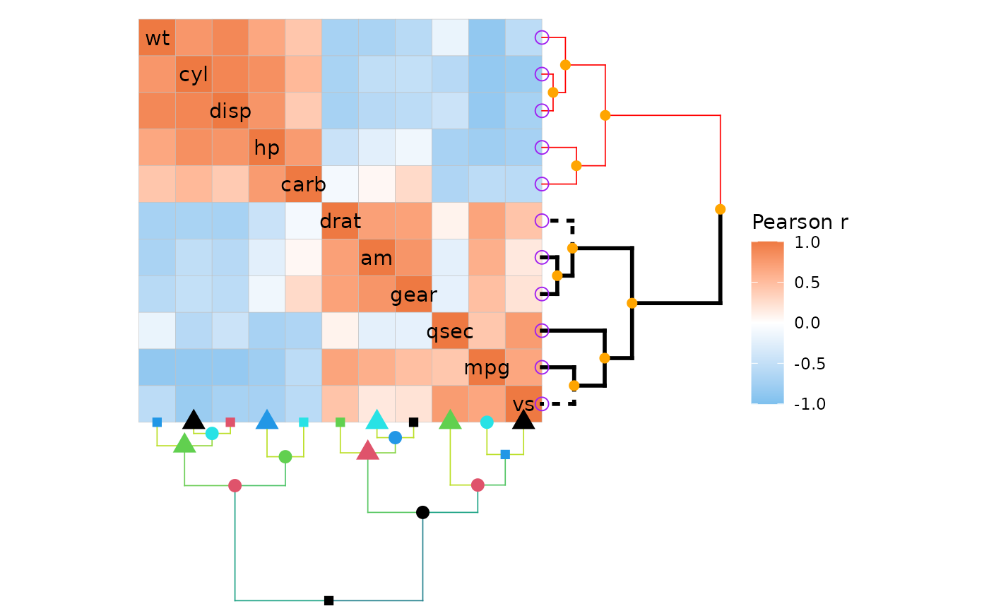

Leaves can be reordered using functions like ladderize or rotate, though it is not recommended to do for only one dimension if the matrix is square as the diagonal may end up in strange places. In such cases, triangular layouts are not supported.

plt1 <- gghm(scale(mtcars[11:15, ]), cluster_rows = TRUE, na_remove = TRUE) # Remove NaNs introduced by scaling
plt2 <- gghm(scale(mtcars[11:15, ]), cluster_rows = TRUE, na_remove = TRUE,
             # dendextend::rotate() to flip the order of rows
             dend_rows_extend = . %>% rotate(5:1))

plt1 / plt2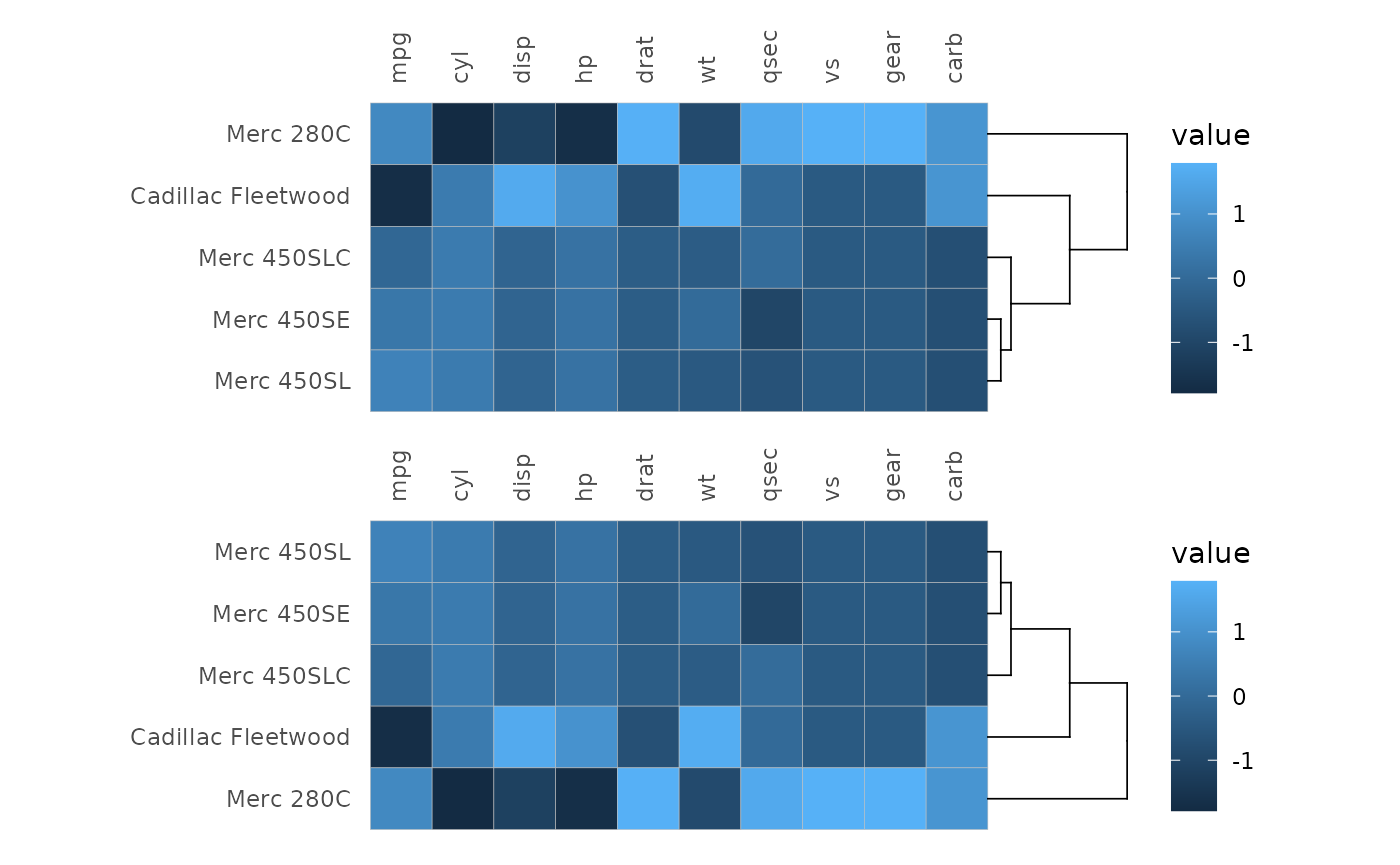

Two heatmaps of rows 11 to 15 of mtcars. Both have clustered rows, but the second plot has its rows in the opposite order compared to the first plot.

# Only the rows are reordered, causing the matrix to become asymmetric
# If the layout were triangular (or mixed), the warning would be slightly different
# and the same plot as below would be produced (forced full layout).
ggcorrhm(mtcars, cluster_rows = TRUE, cluster_cols = TRUE,
         dend_rows_extend = list(ladderize = NULL))
#> Warning: The clustering has ordered rows and columns differently. The diagonal may be
#> scrambled due to the unequal row and column orders.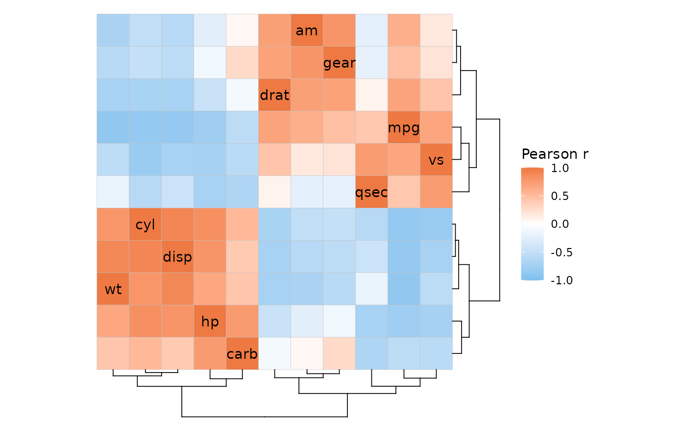

Correlation heatmap of mtcars. Both the rows and columns are clustered, but the dendrograms have ordered the data differently causing the cells that would normally lie on the diagonal to be spread away from the diagonal. Those cells are still labelled with the column names.

Finally, since cluster_rows and cluster_cols can take dendrogram objects, it is possible to do the dendextend customisation externally. dend_rows_extend and dend_cols_extend are applied on top of that, meaning that the two approaches can be combined.

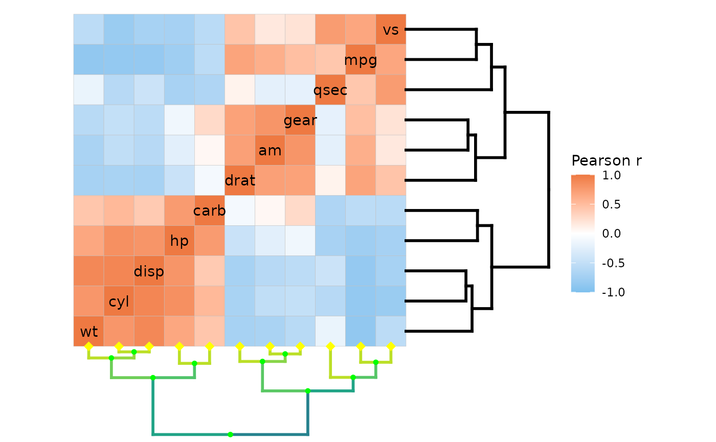
# Cluster data before
clust1 <- mtcars %>% cor() %>% dist() %>% hclust() %>% as.dendrogram()
# Apply some dendextend functions
clust2 <- clust1 %>% highlight_branches_col() %>%
  set("nodes_pch", 20) %>% set("nodes_col", "green") %>% set("nodes_cex", 2) %>%
  set("leaves_pch", 18) %>% set("leaves_col", "yellow") %>% set("leaves_cex", 3)

ggcorrhm(mtcars, cluster_rows = clust1, cluster_cols = clust2,
         # Increase height and linewidth for visibility
         dend_height = .6, dend_lwd = 1,
         # Apply some customisation to the row dendrogram too
         dend_rows_extend = . %>% raise.dendrogram(3) %>%
           # Rotating the row dendrogram of a symmetric matrix to be in the
           # reverse order will give a diagonal that runs from the bottom left
           # to the top right, but a warning will still be produced. Mixed layouts 
           # allow for such diagonals without warnings
           rotate(11:1))
#> Warning: The clustering has ordered rows and columns differently. The diagonal may be
#> scrambled due to the unequal row and column orders.

A mtcars correlation heatmap with clustered rows and columns. The diagonal runs from bottom left to top right. The dendrograms have thick lines, and the lowest split in the row dendrogram has been raised. The column dendrogram colours shift from dark green to yellow the closer to the heatmap it gets and the nodes are green circles while the leaves are yellow diamonds.

Dendrogram position

Changing how the dendrograms look

More customisation using dendextend

More customisation using `dendextend`