Scales and legends • ggcorrheatmap

library(ggcorrheatmap)
library(ggplot2)
library(patchwork)  # Arrange plots and legends
library(cowplot)    # For extracting and arranging legends

Scales

As explained in some of the other articles, the colour scale argument col_scale takes NULL (for default scales), a character (for Brewer and Viridis scales) and ggplot2 scale objects. When passing scale objects, make sure the correct aesthetic is used (fill or colour/color depending on plotting mode).

plt1 <- gghm(volcano, col_name = "Default",
             border_col = NA, show_names_x = FALSE, show_names_y = FALSE)

plt2 <- gghm(volcano,
             # Brewer Spectral palette
             col_scale = "A", col_name = "Character",
             border_col = NA, show_names_x = FALSE, show_names_y = FALSE)

plt3 <- gghm(volcano,
             # Custom scale
             col_scale = scale_fill_gradient2(
               high = "pink", mid = "white", low = "lightblue",
               midpoint = 140, name = "Custom"
             ),
             border_col = NA, show_names_x = FALSE, show_names_y = FALSE)

plt1 + plt2 + plt3 &
  theme(legend.position = "bottom",
        legend.title = element_text(vjust = 0.8))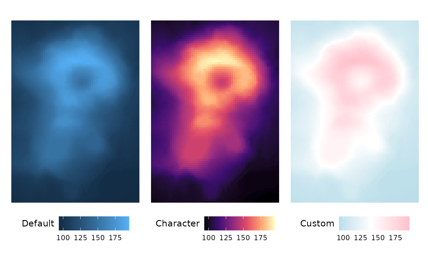

Three heatmaps of the volcano data. The first one uses the default dark blue to light blue gradient for the cells, the second one uses the Viridis magma palette, and the third a custom scale going from light blue to white to pink.

This is also true for the annotation scale arguments annot_rows_col and annot_cols_col.

row_annot <- data.frame(.names = rownames(mtcars)[1:10],
                        Default = 1:10,
                        Character = 1:10,
                        Custom = 1:10)

row_annot_fill <- list(Default = NULL,
                       Character = "Spectral",
                       Custom = scale_fill_gradient2(
                         high = "pink", mid = "white", low = "lightblue",
                         midpoint = 6
                       ))

gghm(mtcars[1:10, 1:5],
     annot_rows_df = row_annot,
     annot_rows_col = row_annot_fill,
     # Make annotation larger and hide heatmap legend
     annot_size = 1,
     legend_order = c(NA, 1:3)) +
  theme(plot.margin = margin(0, 0, 30, 0))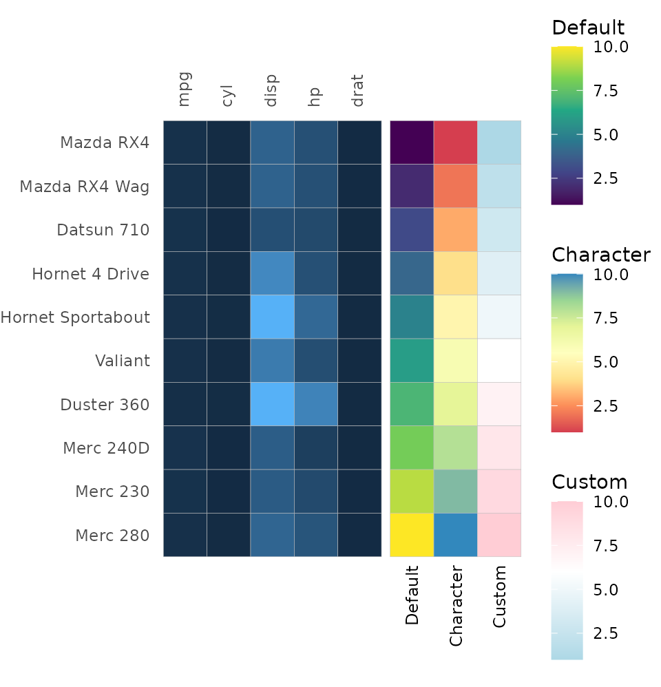

A heatmap of the first ten rows and five columns of mtcars. Three row annotations can be seen on the right side, the first one using the Viridis scale, the second one the Brewer Spectral, and the third one a custom scale going from light blue to white to pink.

When col_scale is a character, “rev_” or “_rev” can be added to the beginning or end, respectively, to reverse the scale. This also works for annotation scales.


row_annot <- data.frame("Default" = 1:nrow(volcano),
                        "Reversed" = 1:nrow(volcano))
row_annot_colr <- list("Default" = "A", "Reversed" = "A_rev")

gghm(volcano, show_names_x = FALSE, show_names_y = FALSE, border_col = NA,
     col_scale = "rev_A", col_name = "Reversed",
     annot_rows_df = row_annot,
     annot_rows_col = row_annot_colr,
     # Make the annotation larger for visibility
     annot_size = 3, annot_dist = 1.5) +
  # Change the margins a bit too
  theme(plot.margin = margin(0, 0, 40, 0))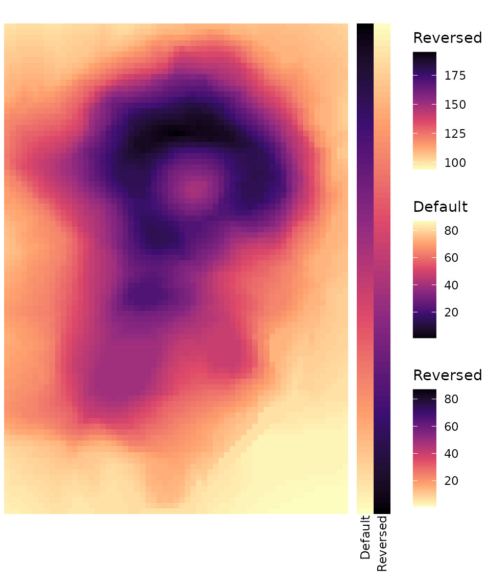

A heatmap of the volcano data with cells coloured using the Viridis magma palette but reversed so that low values are light and high are dark. Two row annotations are seen to the right, both have the same values but one is using the default magma palette and the other the reversed one.

The default scale for the main heatmap is different for ggcorrhm() as it assumes that correlations are plotted. There are also more arguments to modify the scale, such as the colours or binning.

When the plot is using a mixed layout, col_scale can also take a vector or list to apply different scales to the different triangles.

plt_dat <- sapply(1:10, function(x) seq(x, x + 9))

gghm(plt_dat, layout = c("tl", "br"),
     mode = c("hm", "hm"),
     # For Viridis options, both the short and long versions work
     col_scale = c("magma", "RdYlGn"))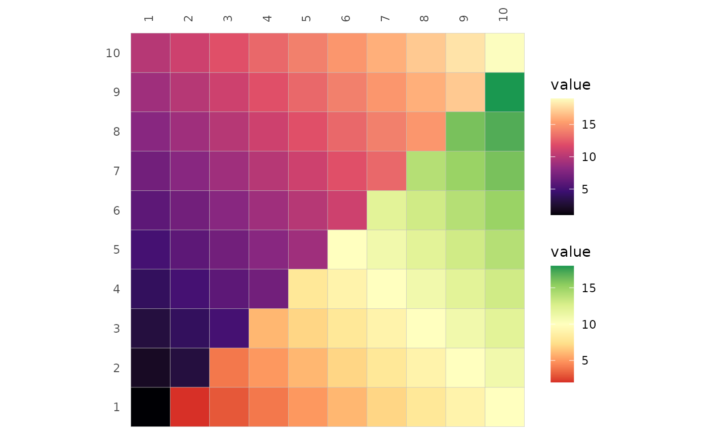

A heatmap of a 10x10 matrix with values arranged so that there is a gradient across the heatmap with low values in the bottom left and high values in the top right. The top left triangle uses the Viridis magma scale, while the bottom right triangle is using the Brewer RdYlGn palette.

col_scale can still be one value to apply the same scale to both triangles. This does not work for scale objects, as the two triangles may use different aesthetics (fill or colour). This means that there will be two colour legends for the main heatmap if the two triangles use different aesthetics, even if they use the same colours. ggcorrhm() hides one of the legends by default and the legend order section goes into more detail on how this can be done.

gghm(plt_dat, layout = c("tl", "br"),
     mode = c("hm", "text"), col_scale = "A")

A heatmap of the same gradient data as the previous figure. The bottom right triangle now has coloured numbers (cell values) in the cells, using the same colour palette (Viridis magma) as the top left triangle. Two legends showing the same values and scale are on the right.

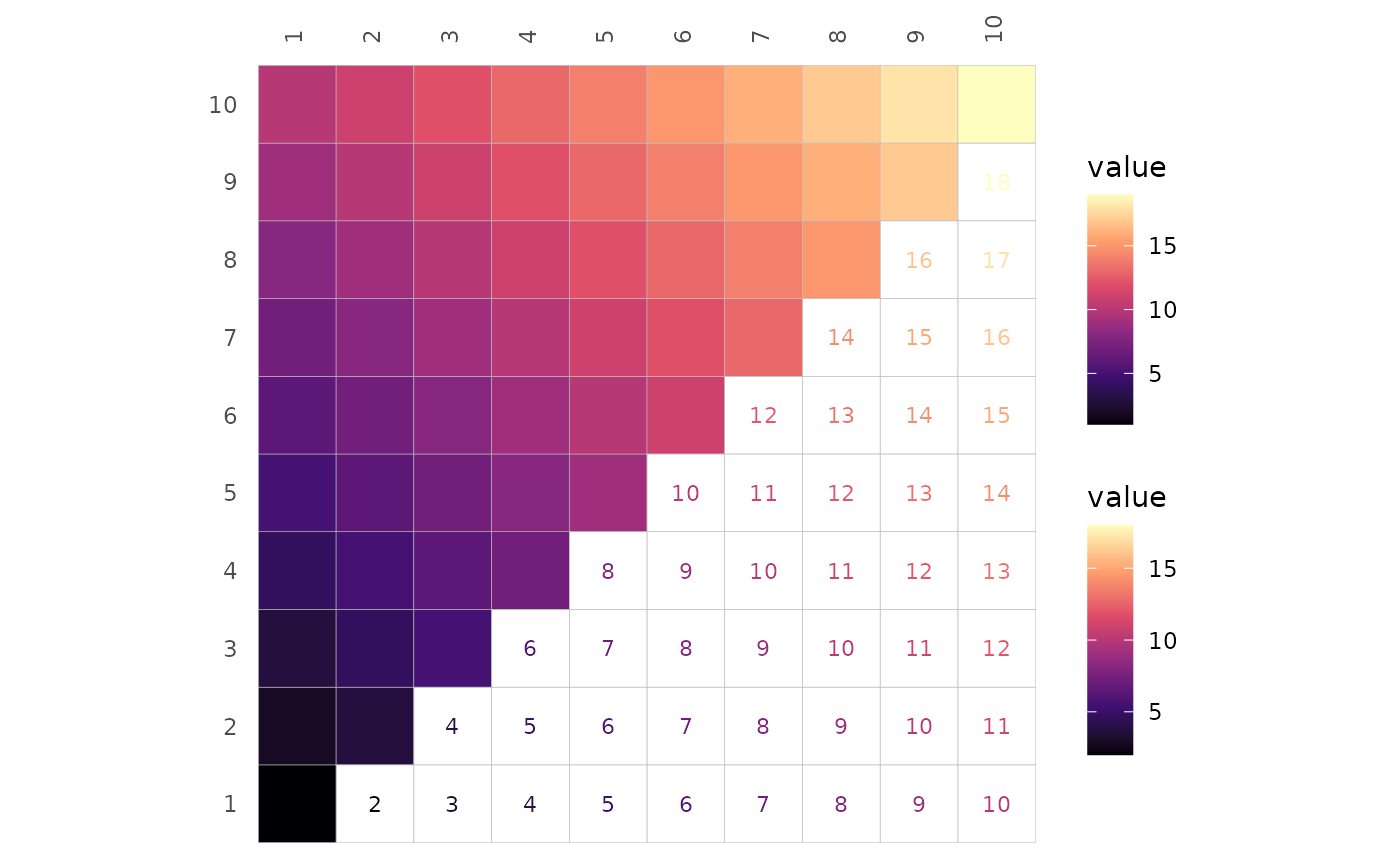
As also explained in the mixed layout article, the scale-modifying arguments bins, na_col, limits, and in ggcorrhm() also high, mid, low, midpoint, and size_range can be applied triangle-wise. If only one scale is provided but a scale-modifying argument is applied differently per triangle, two scales are created anyway.

# Only one scale supplied, but it is split into two by
# specifying two different binnings
gghm(plt_dat, layout = c("tr", "bl"), mode = c("hm", "hm"),
     col_scale = "G", bins = c(4L, 8L))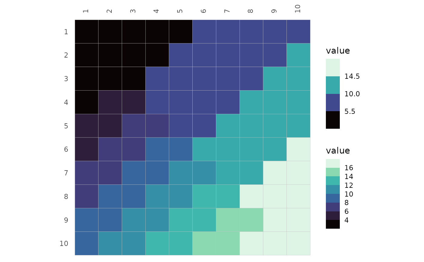

A 10x10 heatmap showing a gradient of values going from low values (starting at 1) in the top left to high values (up to 19) in the bottom right. The Viridis mako colour scale is used, shifting from black (low values) through blue and teal and ending at a pale green. The top right triangle of the heatmap is divided in to four bins while the bottom left triangle has eight.

When using scale objects, arguments that change scales and legends such as col_name or legend_order and, for ggcorrhm(), high, mid, low etc will be ignored to instead give the user full control. This allows for more flexibility, such as changing the breaks, bin sizes, or changing how out of bounds values are treated.

The default way ggplot2 deals with values outside of the scale range (out of bound value) is to replace them with NAs. The oob argument of the scale functions can change the behaviour, e.g. so that OOB values use the extreme colours of the scale.

# Normal limits
plt1 <- gghm(plt_dat, col_scale = "RdYlGn_rev",
             cell_labels = TRUE)

# Narrower limits with handling of oob values
plt2 <- gghm(plt_dat, layout = c("tr", "bl"),
     mode = c("hm", "hm"),
     col_scale = list(
       # scale_fill_distiller to use Brewer palettes with continuous data
       # The default direction in distiller is -1, opposite of gghm
       scale_fill_distiller(
         palette = "RdYlGn",
         # Values outside the limits are replaced with NAs
         limits = c(7, 13),
         # Can then change the colour using the na.value argument
         # (corresponding to na_col in gghm)
         na.value = "beige"
       ),
       
       scale_fill_distiller(
         palette = "RdYlGn",
         limits = c(7, 13),
         # Change oob strategy 'oob' argument
         # scales::squish assigns the extreme colours to values outside the range
         oob = scales::squish
       )
     ), cell_labels = TRUE)

plt1 + plt2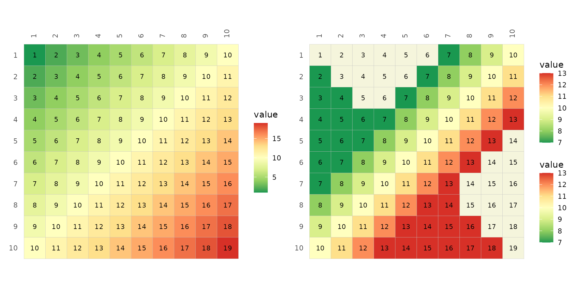

When binning scales with the bins argument, a number of the ‘double’ class will prioritise breaks at nice numbers while an integer will prioritise the number of bins. As a side note, out-of-bound values with binned scales also default to using the ‘squish’ strategy shown above.


# Make plot data between -1 and 1 (like correlation data)
plt_dat_cor <- sapply(seq(-1, 0, length.out = 100), function(x) {
  seq(x, x + 1, length.out = 100)
})

# Simple mixed layout with mixed scales
plt1 <- ggcorrhm(plt_dat_cor, cor_in = TRUE, show_names_diag = FALSE,
                 border_col = 0, layout = c("tl", "br"), mode = c("hm", "hm"),
                 col_scale = c("Spectral", "H"))

# With many scale arguments applied
plt2 <- ggcorrhm(plt_dat_cor, cor_in = TRUE, show_names_diag = FALSE,
                 border_col = 0, layout = c("tl", "br"), mode = c("hm", "hm"),
                 col_scale = c("Spectral", "H"),
                 # Provide a list as a mix of integer and float would be coerced if atomic vector
                 # Integer vs double, results in 11 and 10 bins
                 bins = list(11L, 11),
                 # NULL to use default limits (-1 to 1 in ggcorrhm)
                 limits = list(c(-.5, .5), NULL))

plt1 + plt2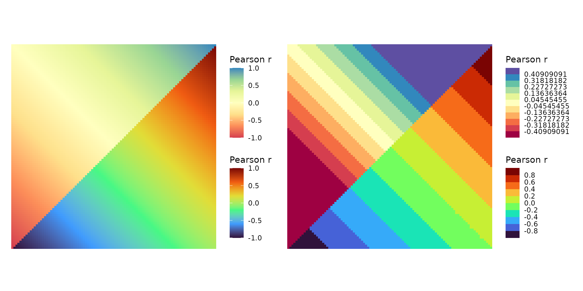

By using scale objects, breaks in both continuous and binned scales can be put wherever desired.


plt_dat_cor <- sapply(seq(-1, 0, length.out = 10), function(x) {
  seq(x, x + 1, length.out = 10)
})

plt1 <- ggcorrhm(plt_dat_cor, cor_in = TRUE)

plt2 <- ggcorrhm(plt_dat_cor, cor_in = TRUE,
                 layout = c("tr", "bl"),
                 mode = c("hm", "hm"),
                 col_scale = list(
                   scale_fill_gradient2(
                     # Mimic the default correlation scale
                     high = "sienna2", mid = "white", low = "skyblue2",
                     # If not binned this only changes the legend but not the colours
                     breaks = seq(-1, 1, length.out = 11)
                   ),
                   # Binned scales can be made with e.g.
                   # scale_fill_fermenter, scale_fill_viridis_b, scale_fill_steps etc
                   scale_fill_steps2(
                     high = "sienna2", mid = "white", low = "skyblue2",
                     # Specify exact break points for bins
                     breaks = c(-1, -0.75, -0.25, 0, 0.25, 0.75, 1)
                   )
                 ))

plt1 + plt2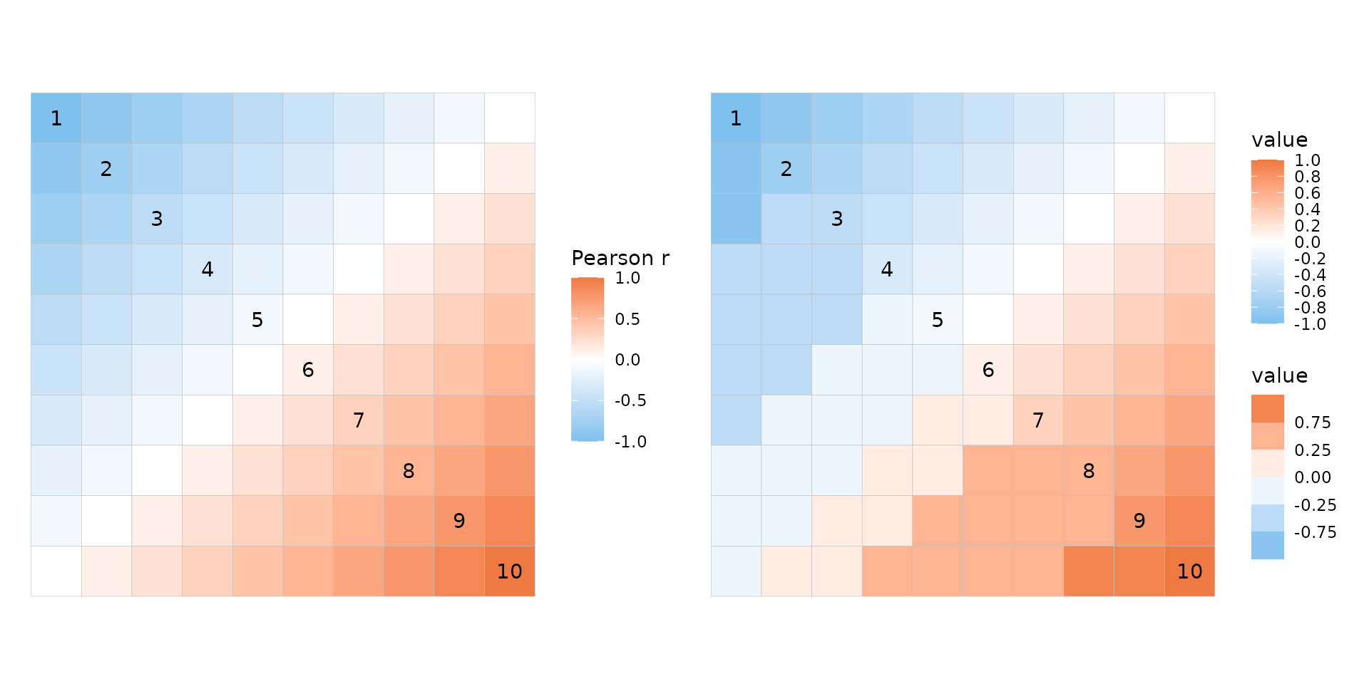

Size scales can be customised as well. ggcorrhm() uses an absolute value transform for the default size scale and hides the legend as it becomes inaccurate (as can be seen in the plot below). scale_size_area can be passed to size_scale to still scale with the absolute value and keep a meaningful legend, at the cost of not being able to set the lower limit for the sizes.

ggcorrhm(mtcars, layout = c("tr", "bl"), mode = c(23, 23),
         size_scale = list(
           # Can make a binned size scale
           scale_size_binned(n.breaks = 6, range = c(2, 6),
                             # Absolute value transform but legend loses meaning
                             transform = scales::trans_new("abs", abs, abs),
                             name = "scale_size_binned\n(absolute value)",
                             guide = guide_bins(order = 1)),
           # scale_size_area, scale_size_binned_area also scale with absolute value
           # but fewer options to control sizes
           scale_size_area(max_size = 10, name = "scale_size_area")
         ), border_lwd = 1, legend_order = NA)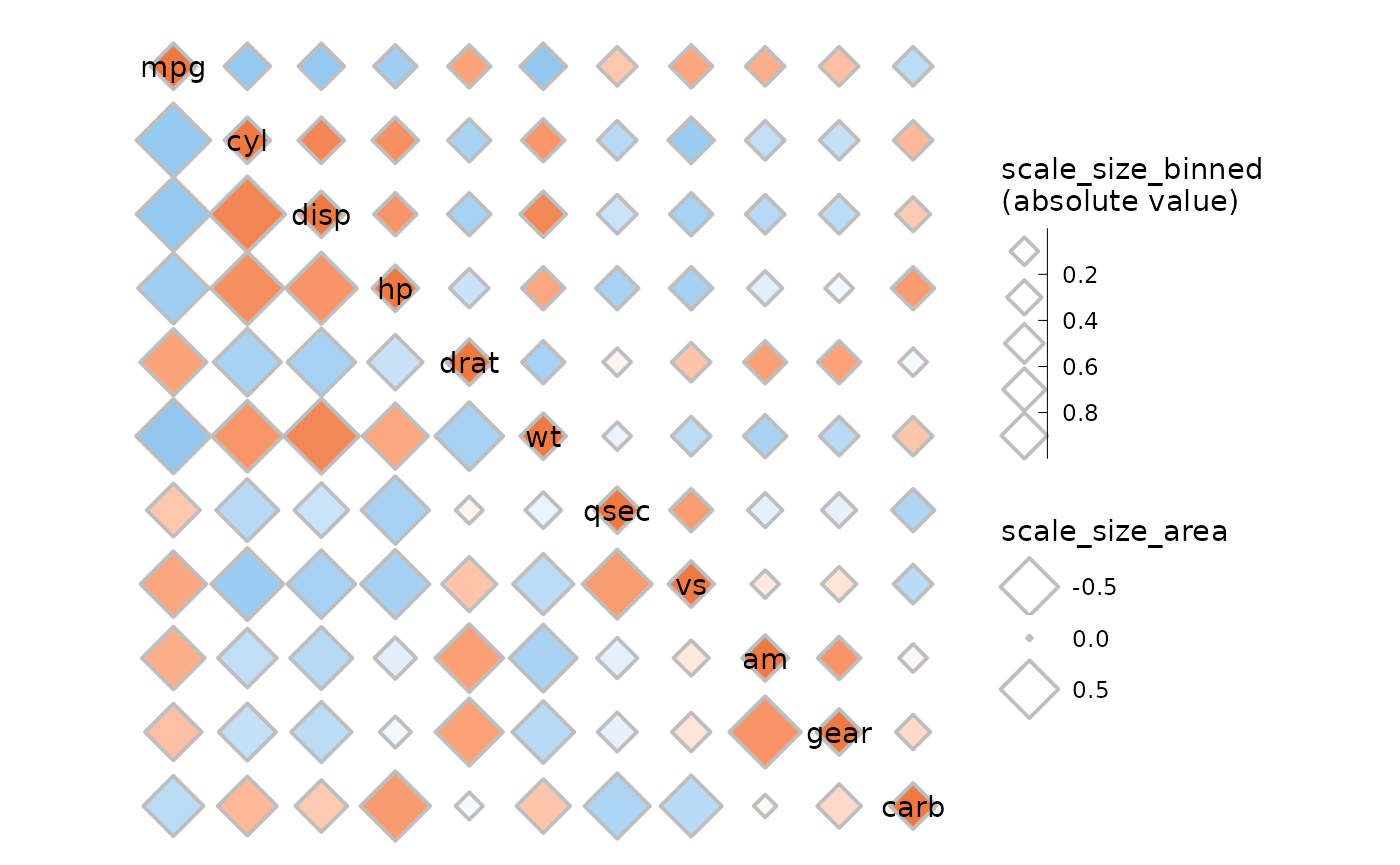

mtcars correlation heatmap with diamonds instead of cells. In the top right triangle the diamonds are smaller than in the bottom left. The sizes of all diamonds scale with the absolute value of the correlations, but the legend for the top right diamonds goes from 0 to 1 while the legend for the other triangle properly shows the negative values too.

Legend order

Legends have a set default order:

Main heatmap colours.
Main heatmap sizes.
Row annotations in order.
Column annotations in order.

row_annot <- data.frame(.names = rownames(mtcars)[1:10], 1:10)
colnames(row_annot)[2] <- "3"

col_annot <- data.frame(.names = colnames(mtcars), 11:1)
colnames(col_annot)[2] <- "4"

gghm(scale(mtcars)[1:10, ], mode = 23,
     col_name = "1", size_name = "2",
     annot_rows_df = row_annot,
     annot_cols_df = col_annot) +
  # Make the legends horizontal to fit better
  theme(legend.direction = "horizontal")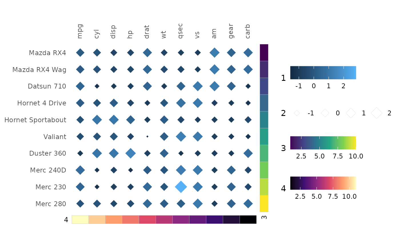

If the layout is mixed, the legends of the first triangle appear before those of the second triangle.

gghm(cor(mtcars), layout = c("tr", "bl"), mode = c("15", "hm"),
     col_scale = c("H", "A"), col_name = c("Triangle 1", "Triangle 2"),
     size_name = "Triangle 1") +
  theme(legend.direction = "horizontal")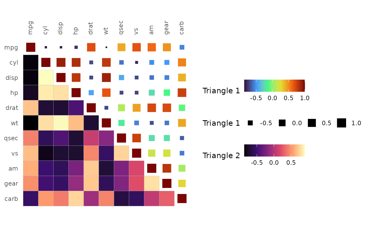

mtcars correlation heatmap with cells in the bottom left triangle and squares with sizes varying with the value in the top right. The deafult ggplot2 colour scale (dark blue to light blue) is used for both triangles. Three legends are on the right, the first one a colour scale, the second one a size scale, and the third one another colour scale.

The order can be changed by using the legend_order argument. This argument takes a numeric vector, the first element specifying the order for the first legend (of the default order), the second element for the second legend and so on. If a value is NA, that legend is hidden.

set.seed(123)
annot_rows <- data.frame(.names = colnames(mtcars), 1:11, 11:1)
colnames(annot_rows)[2:3] <- c("4", "5")
annot_cols <- data.frame(.names = colnames(mtcars),
                         sample(letters[1:3], 11, TRUE),
                         sample(LETTERS[1:2], 11, TRUE))
colnames(annot_cols)[2:3] <- c("6", "7")

plt1 <- gghm(cor(mtcars), layout = c("tl", "br"), mode = c(19, 21),
             col_name = c("1", "3"), size_name = c("2"),
             annot_rows_df = annot_rows,
             annot_cols_df = annot_cols)

plt2 <- gghm(cor(mtcars), layout = c("tl", "br"), mode = c(19, 21),
             col_name = c("1", "3"), size_name = c("2"),
             annot_rows_df = annot_rows,
             annot_cols_df = annot_cols,
             legend_order = c(4, 2, NA, 1, 5, NA, 3))

plt1 / plt2 &
  theme(legend.direction = "horizontal")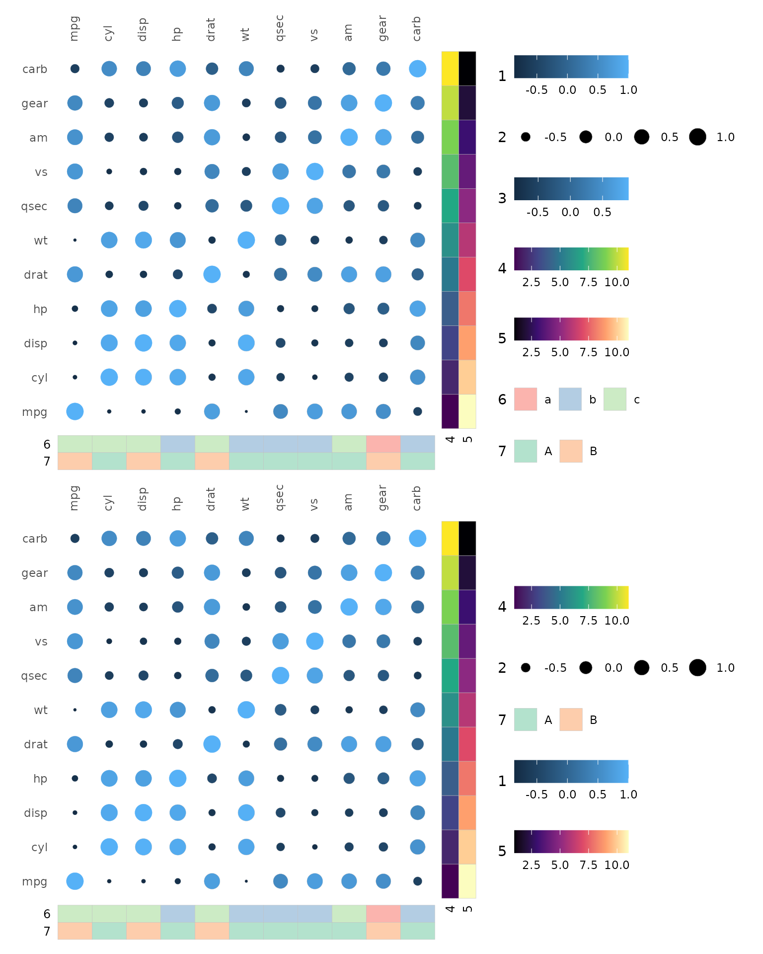

Two mtcars correlation heatmaps with circles instead of cells. Both have two row and two column annotations each. The first heatmap has seven legends on the right (colour, size, colour, row annotation colours 1-2, column annotation colours 1-2), named 1 to 7. The second heatmap is the same as the first but with the legends ordered 4, 2, 7, 1, 5. The 3 and 6 legends are missing.

A single NA value hides all legends.

gghm(cor(mtcars), layout = c("tl", "br"), mode = c(19, 21),
     col_name = c("1", "3"), size_name = c("2"),
     annot_rows_df = annot_rows,
     annot_cols_df = annot_cols,
     legend_order = NA)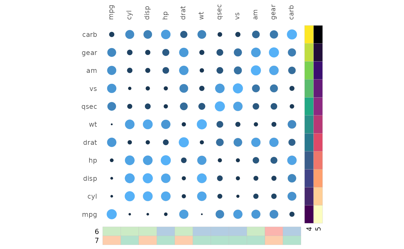

The mtcars correlation heatmap with circles as above, but with no legends.

Scales can be specified as ggplot2 scale objects. In this case the user has complete control over the scale and it is unaffected by arguments like legend_order or col_name.

gghm(cor(mtcars), layout = c("tl", "br"), mode = c(19, 21),
     col_name = c("1", "3"), size_name = "2",
     col_scale = list(
       # Keep default scale for first triangle
       NULL,
       # Pass a scale object for second triangle
       scale_fill_viridis_c(name = "scale object 1", option = "G",
                            guide = guide_colourbar(order = 1))
     ),
     annot_rows_df = annot_rows,
     annot_cols_df = annot_cols,
     annot_rows_col = list(
       # Scale object for second row annotation
       "5" = scale_fill_distiller(name = "scale object 2",
                                  palette = "Purples")
     ),
     annot_cols_col = list(
       # Scale object for first column annotation
       "6" = scale_fill_brewer(name = "scale object 3",
                               palette = "RdBu",
                               # Hide the legend
                               guide = "none")
     ),
     # (Try to) Remove all legends
     legend_order = NA) +
  theme(legend.direction = "horizontal")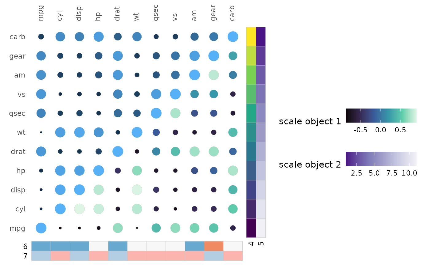

Legends in correlation heatmaps

ggcorrhm() tries to hide some legends by default when using mixed layouts to reduce clutter.

For example, when both triangles use the same colour scale, one of the scales is hidden. This only happens when the default scale is used (customised with high, mid, etc is ok) or when col_scale is a character. If col_scale contains ggplot2 scale objects both legends will be shown (unless specified not to in the scale object).

Default size legends are also hidden as they use an absolute value transformation and show different information from the colour scale.

# If both triangles use the same colour scale
# (when col_scale is NULL or a one character value)
ggcorrhm(mtcars, layout = c("tl", "br"),
         mode = c("hm", "18"), col_scale = "RdYlBu")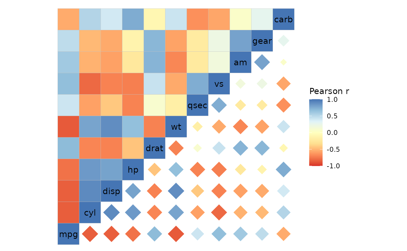

mtcars correlation heatmap with cells in the top left and diamonds in the bottom right. The heatmap uses the Brewer RdYlBu scale that ranges from blue to yellow to red. There is only one legend on the right, showing the colour scale.

The legends can be included again by using the legend_order argument or using scale objects for the scales.

ggcorrhm(mtcars, layout = c("tl", "br"),
         mode = c("hm", "18"), col_scale = "RdYlBu",
         # Elements beyond the number of legends are ignored
         # On a related note, if legend_order is shorter than
         # the number of legends, legends not in the vector are hidden
         legend_order = 1:10)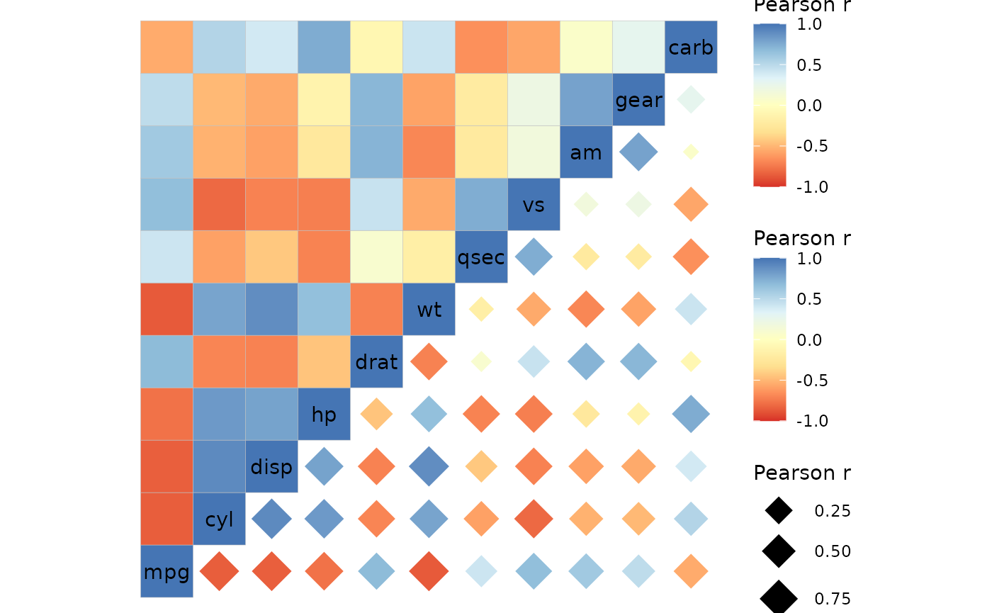

mtcars correlation heatmap with cells and diamonds and the RdYlBu scale like above. There are three legends one the right, the first two for the colour scale and the last one for the sizes (showing the absolute values).

Arranging legends

When there are many legends, some of them may be cut off and it can be tricky to make them fit. One way is to change the positions, sizes or orientations of legends as shown in some of the plots above. Another way is to change the size of the figure until the legends fit. A more advanced way is to use packages like cowplot and patchwork to stitch together a legend-less version of the plot with the legends, which also makes it possible to arrange the legends in grids.


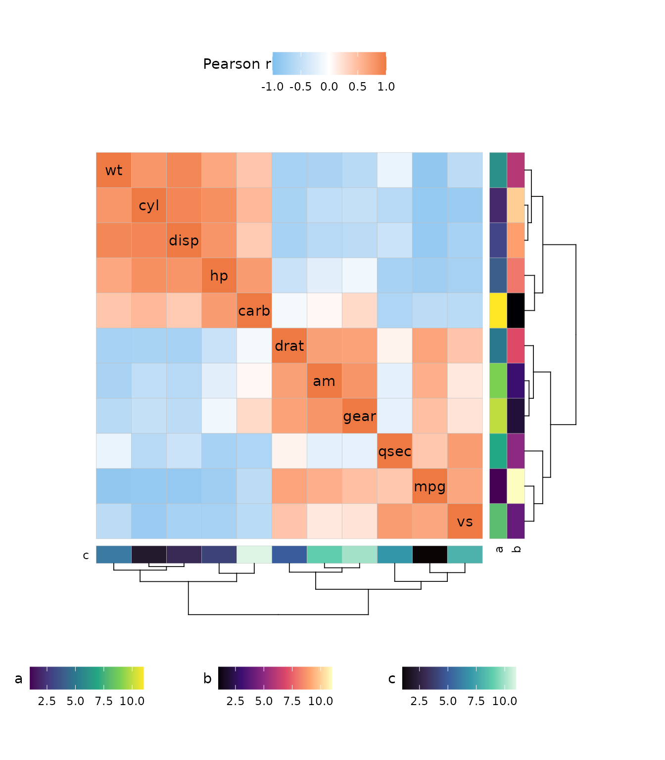
# Plot with legends
p <- ggcorrhm(mtcars, cluster_rows = TRUE, cluster_cols = TRUE,
              annot_rows_df = data.frame(.names = colnames(mtcars),
                                         a = 1:11, b = 11:1),
              annot_cols_df = data.frame(.names = colnames(mtcars),
                                         c = 1:11))

# Plot without legends
pl <- ggcorrhm(mtcars, cluster_rows = TRUE, cluster_cols = TRUE,
               annot_rows_df = data.frame(.names = colnames(mtcars),
                                          a = 1:11, b = 11:1),
               annot_cols_df = data.frame(.names = colnames(mtcars),
                                          c = 1:11),
               legend_order = NA)

# Show plot with default legends
p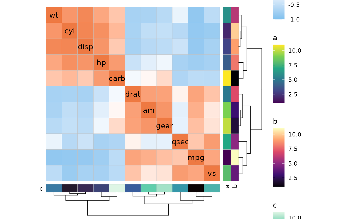

mtcars correlation heatmap with clustered rows and columns, as well as two row annotations and one column annotation. Four legends can be seen to the right, but they do not all fit and the first and last one cannot be seen fully.

# Extract the four legends
lgd <- get_legend(p)[["grobs"]][1:4]

# Arrange in a grid (cowplot)
lgd_grid <- plot_grid(plotlist = lgd, nrow = 2, ncol = 2)

# Combine legend-less plot and legends with cowplot
plot_grid(pl, lgd_grid, rel_widths = c(3, 1))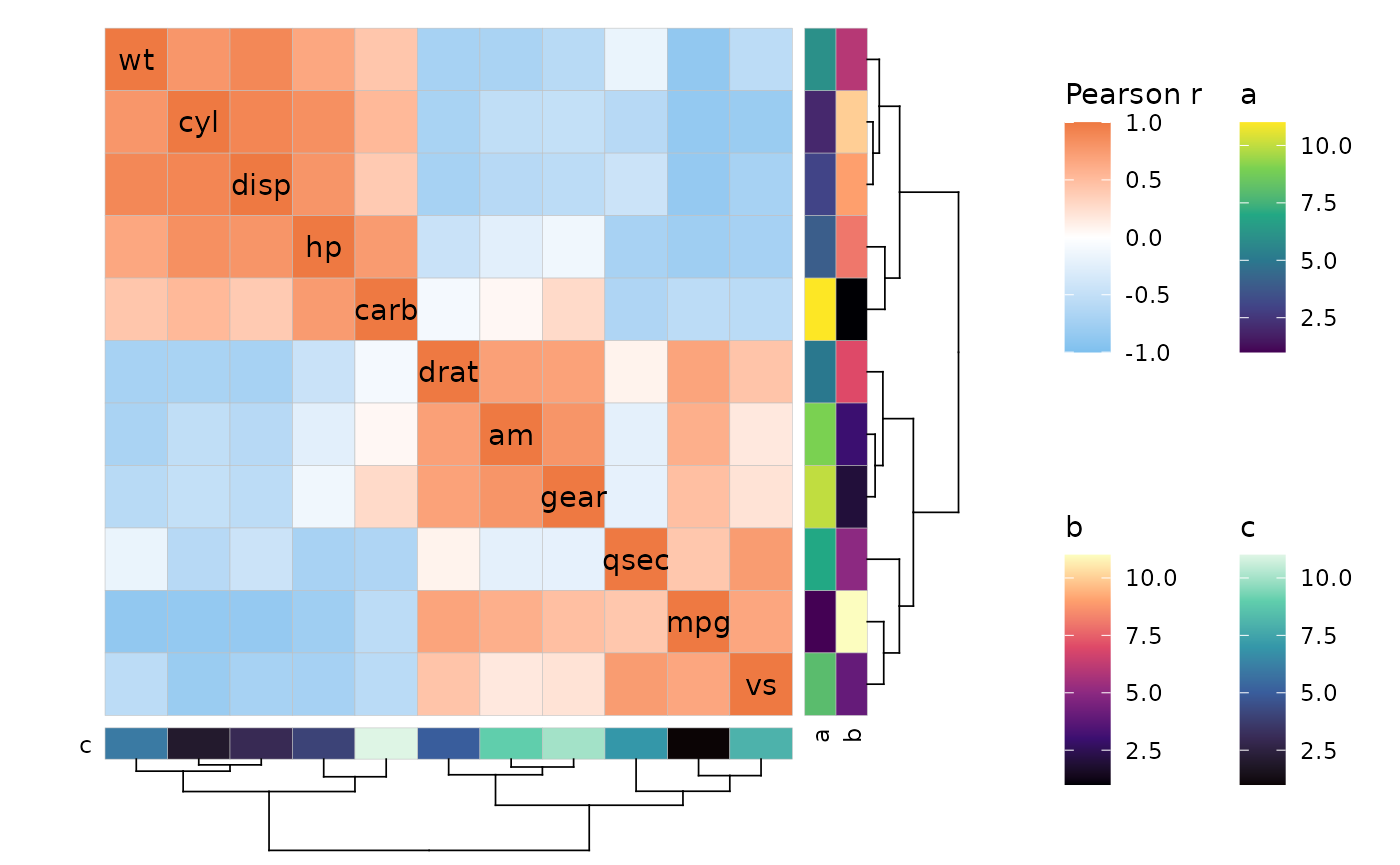

The same heatmap with annotations as the previous figure, but the legends are now all visible, arranged in a 2x2 grid to the right of the plot.


# Code for the same layout as above
# # Arrange in a grid (patchwork)
# lgd_grid <- wrap_plots(lgd)
# 
# # Combine with patchwork
# wrap_plots(pl, lgd_grid, widths = c(3, 1))

# Try a different layout with patchwork. Turn the legends horizontal
lgd <- get_legend(p + theme(legend.direction = "horizontal",
                            legend.title = element_text(vjust = 0.8)))[["grobs"]][1:4]

# Append the plot to the legend list to give to patchwork::wrap_plots
wrap_plots(append(list(pl), lgd),
           design = "
           ##BBB##
           AAAAAAA
           AAAAAAA
           AAAAAAA
           AAAAAAA
           CCDDEEE
           ")

The same heatmap as the previous plot. The legends are now horizontal and split into two groups, the Pearson r legend above and the annotation legends below the heatmap.